The CUBE operator in the GROUP BY clause analyzes data by forming the data into groups in more than one dimension (grouping expression).
CUBE requires an ordered list of dimensions as arguments and enables the SELECT statement to calculate subtotals for all possible combinations of the group of dimensions that you specify in the query and generates a result set that shows aggregates for all combinations of values in selected columns.
SELECT … [ GROUPING (column-name) … ] …
GROUP BY [ expression [,…]
| CUBE ( expression [,…] ) ]
GROUPING takes a column name as a parameter, and returns a Boolean value as listed in the following table:
If the value of the result is |
GROUPING returns |
|---|---|
NULL created by a CUBE operation |
1 (TRUE) |
NULL indicating the row is a subtotal |
1 (TRUE) |
Not created by a CUBE operation |
0 (FALSE) |
A stored NULL |
0 (FALSE) |
CUBE is particularly useful when your dimensions are not a part of the same hierarchy.
This SQL syntax... |
Defines the following sets... |
|---|---|
GROUP BY CUBE (A, B, C); |
(A, B, C) (A, B) (A, C) (A) (B, C) (B) (C) ( ) |
The CUBE operator supports all of the aggregate functions available to the GROUP BY clause, but CUBE is currently not supported with COUNT DISTINCT or SUM DISTINCT.
CUBE is currently not supported with the inverse distribution analytical functions, PERCENTILE_CONT and PERCENTILE_DISC.
CUBE can only be used in the SELECT statement; you cannot use CUBE in a SELECT subquery.
A GROUPING specification that combines ROLLUP, CUBE, and GROUP BY columns in the same GROUP BY clause is not currently supported.
Constant expressions as GROUP BY keys are not supported.
GROUPING can be used with the CUBE operator to distinguish between stored NULL values and NULL values in query results created by CUBE.
See the examples in the description of the ROLLUP operator for illustrations of the use of the GROUPING function to interpret results.
All CUBE operations return result sets with at least one row where NULL appears in each column except for the aggregate columns. This row represents the summary of each column to the aggregate function.
CUBE example 1—The following queries use data from a census, including the state (geographic location), gender, education level, and income of people. The first query contains a GROUP BY clause that organizes the results of the query into groups of rows, according to the values of the columns state, gender, and education in the table census and computes the average income and the total counts of each group. This query uses only the GROUP BY clause without the CUBE operator to group the rows.
SELECT State, Sex as gender, DepartmentID, COUNT(*),CAST(ROUND(AVG(Salary),2) AS NUMERIC(18,2))AS AVERAGEFROM employees WHERE state IN ('MA' , 'CA')GROUP BY State, Sex, DepartmentIDORDER BY 1,2;
The results from the above query:
state  gender  DepartmentID  COUNT()     AVERAGE
-----  ------  -------   --------    --------
CA       F       200       2         58650.00
CA       M       200       	1         39300.00
Use the CUBE extension of the GROUP BY clause, if you want to compute the average income in the entire census of state, gender, and education and compute the average income in all possible combinations of the columns state, gender, and education, while making only a single pass through the census data. For example, use the CUBE operator if you want to compute the average income of all females in all states, or compute the average income of all people in the census according to their education and geographic location.
When CUBE calculates a group, a NULL value is generated for the columns whose group is calculated. The GROUPING function must be used to distinguish whether a NULL is a NULL stored in the database or a NULL resulting from CUBE. The GROUPING function returns 1 if the designated column has been merged to a higher level group.
CUBE example 2—The following query illustrates the use of the GROUPING function with GROUP BY CUBE.
SELECT case grouping(State) WHEN 1 THEN 'ALL' ELSE StateEND AS c_state, case grouping(sex) WHEN 1 THEN 'ALL'ELSE Sex end AS c_gender, case grouping(DepartmentID)WHEN 1 THEN 'ALL' ELSE cast(DepartmentID as char(4)) endAS c_dept, COUNT(*), CAST(ROUND(AVG(salary),2) ASNUMERIC(18,2))AS AVERAGEFROM employees WHERE state IN ('MA' , 'CA')GROUP BY CUBE(state, sex, DepartmentID)ORDER BY 1,2,3;
The results of this query are shown below. The NULLs generated by CUBE to indicate a subtotal row are replaced with ALL in the subtotal rows, as specified in the query.
c_state   c_gender  c_dept    COUNT()   AVERAGE
-------   --------  -------    -----     --------
ALL       ALL        200         3       52200.00
ALL       ALL        ALL         3       52200.00
ALL       F          200         2       58650.00
ALL       F          ALL         2       58650.00
ALL       M         200          1       39300.00
ALL       M         ALL          1       39300.00
CA        ALL       200          3       52200.00
CA        ALL       ALL          3       52200.00
CA        F         200          2       58650.00
CA        F         ALL          2       58650.00
CA        M         200          1       39300.00
CA        M         ALL          1       39300.00
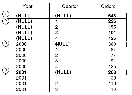
CUBE example 3—In this example, the query returns a result set that summarizes the total number of orders and then calculates subtotals for the number of orders by year and quarter.
SELECT year (OrderDate) AS Year, quarter(OrderDate) AS Quarter, COUNT (*) OrdersFROM SalesOrdersGROUP BY CUBE (Year, Quarter)ORDER BY Year, Quarter
The figure that follows represents the result set from the query. The subtotal rows are highlighted in the result set. Each subtotal row has a NULL in the column or columns over which the subtotal is computed.

The first highlighted row [1] represents the total number of orders across both years and all quarters. The value in the Orders column is the sum of the values in each of the rows marked [3]. It is also the sum of the four values in the rows marked [2].
The next set of highlighted rows [2] represents the total number of orders by quarter across both years. The two rows marked by [3] represent the total number of orders across all quarters for the years 2000 and 2001, respectively.