The following example shows the SUM function used as a window function. The query returns a result set that partitions the data by DepartmentID, and then provides a cumulative summary (Sum_Salary) of employees' salaries, starting with the employee who has been at the company the longest. The result set includes only those employees who reside in California, Utah, New York, or Arizona. The column Sum_Salary provides the cumulative total of employees' salaries.
SELECT DepartmentID, Surname, StartDate, Salary,
SUM( Salary ) OVER ( PARTITION BY DepartmentID
    ORDER BY StartDate
    RANGE BETWEEN UNBOUNDED PRECEDING AND CURRENT ROW )
AS "Sum_Salary"
FROM Employees
WHERE State IN ( 'CA', 'UT', 'NY', 'AZ' )
   AND DepartmentID IN ( '100', '200' )
ORDER BY DepartmentID, StartDate; |
The table that follows represents the result set from the query. The result set is partitioned by DepartmentID.
| DepartmentID | Surname | StartDate | Salary | Sum_Salary | |
|---|---|---|---|---|---|
| 1 | 100 | Whitney | 1984-08-28 | 45700.00 | 45700.00 |
| 2 | 100 | Cobb | 1985-01-01 | 62000.00 | 107700.00 |
| 3 | 100 | Shishov | 1986-06-07 | 72995.00 | 180695.00 |
| 4 | 100 | Driscoll | 1986-07-01 | 48023.69 | 228718.69 |
| 5 | 100 | Guevara | 1986-10-14 | 42998.00 | 271716.69 |
| 6 | 100 | Wang | 1988-09-29 | 68400.00 | 340116.69 |
| 7 | 100 | Soo | 1990-07-31 | 39075.00 | 379191.69 |
| 8 | 100 | Diaz | 1990-08-19 | 54900.00 | 434091.69 |
| 9 | 200 | Overbey | 1987-02-19 | 39300.00 | 39300.00 |
| 10 | 200 | Martel | 1989-10-16 | 55700.00 | 95000.00 |
| 11 | 200 | Savarino | 1989-11-07 | 72300.00 | 167300.00 |
| 12 | 200 | Clark | 1990-07-21 | 45000.00 | 212300.00 |
| 13 | 200 | Goggin | 1990-08-05 | 37900.00 | 250200.00 |
For DepartmentID 100, the cumulative total of salaries from employees in California, Utah, New York, and Arizona is $434,091.69 and the cumulative total for employees in department 200 is $250,200.00.
For more information about the exact syntax of the SUM function, see SUM function [Aggregate].
Using two windows—one window over the current row, the other over the previous row—you can compute deltas, or changes, between adjacent rows. For example, the following query computes the delta (Delta) between the salary for one employee and the previous employee in the results:
SELECT EmployeeID AS EmployeeNumber,
   Surname AS LastName,
   SUM( Salary ) OVER ( ORDER BY BirthDate
      ROWS BETWEEN CURRENT ROW AND CURRENT ROW )
      AS CurrentRow,
   SUM( Salary ) OVER ( ORDER BY BirthDate
      ROWS BETWEEN 1 PRECEDING AND 1 PRECEDING )
      AS PreviousRow,
   ( CurrentRow - PreviousRow ) AS Delta
FROM Employees
WHERE State IN ( 'NY' ); |
| EmployeeNumber | LastName | CurrentRow | PreviousRow | Delta | |
|---|---|---|---|---|---|
| 1 | 913 | Martel | 55700.000 | (NULL) | (NULL) |
| 2 | 1062 | Blaikie | 54900.000 | 55700.000 | -800.000 |
| 3 | 249 | Guevara | 42998.000 | 54900.000 | -11902.000 |
| 4 | 390 | Davidson | 57090.000 | 42998.000 | 14092.000 |
| 5 | 102 | Whitney | 45700.000 | 57090.000 | -11390.000 |
| 6 | 1507 | Wetherby | 35745.000 | 45700.000 | -9955.000 |
| 7 | 1751 | Ahmed | 34992.000 | 35745.000 | -753.000 |
| 8 | 1157 | Soo | 39075.000 | 34992.000 | 4083.000 |
Note that SUM is performed only on the current row for the CurrentRow window because the window size was set to ROWS BETWEEN CURRENT ROW AND CURRENT ROW. Likewise, SUM is performed only over the previous row for the PreviousRow window, because the window size was set to ROWS BETWEEN 1 PRECEDING AND 1 PRECEDING. Also, the value of PreviousRow is NULL in the first row since it has no predecessor, and hence the Delta value is NULL as
well.
Consider the following query, which lists the top salespeople (defined by total sales) for each product in the database:
SELECT s.ProductID AS Products, o.SalesRepresentative,
     SUM( s.Quantity ) AS total_quantity,
     SUM( s.Quantity * p.UnitPrice ) AS total_sales
  FROM SalesOrders o KEY JOIN SalesOrderItems s
    KEY JOIN Products p
  GROUP BY s.ProductID, o.SalesRepresentative
  HAVING total_sales = (
    SELECT First SUM( s2.Quantity * p2.UnitPrice )
        AS sum_sales
      FROM SalesOrders o2 KEY JOIN
        SalesOrderItems s2 KEY JOIN Products p2
      WHERE s2.ProductID = s.ProductID
      GROUP BY o2.SalesRepresentative
      ORDER BY sum_sales DESC )
ORDER BY s.ProductID; |

This query returns the result:
| Products | SalesRepresentative | total_quantity | total_sales | |
|---|---|---|---|---|
| 1 | 300 | 299 | 660 | 5940.00 |
| 2 | 301 | 299 | 516 | 7224.00 |
| 3 | 302 | 299 | 336 | 4704.00 |
| 4 | 400 | 299 | 458 | 4122.00 |
| 5 | 401 | 902 | 360 | 3600.00 |
| 6 | 500 | 949 | 360 | 2520.00 |
| 7 | 501 | 690 | 360 | 2520.00 |
| 8 | 501 | 949 | 360 | 2520.00 |
| 9 | 600 | 299 | 612 | 14688.00 |
| 10 | 601 | 299 | 636 | 15264.00 |
| 11 | 700 | 299 | 1008 | 15120.00 |
The original query is formed using a correlated subquery that determines the highest sales for any particular product, as ProductID is the subquery's correlated outer reference. Using a nested query, however, is often an expensive option, as in this case. This is because the subquery involves not only a GROUP BY clause, but also an ORDER BY clause within the GROUP BY clause. This makes it impossible for the query optimizer to rewrite this nested query as a join while retaining the same semantics.

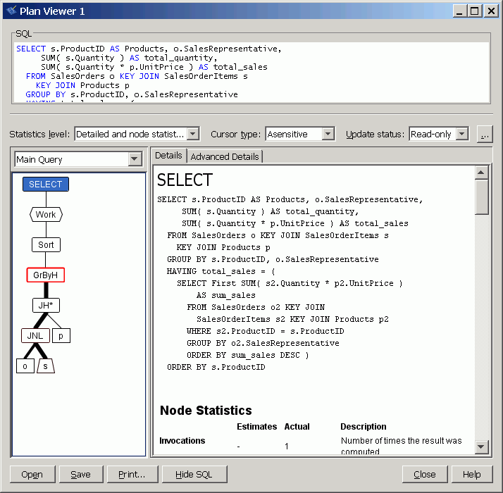
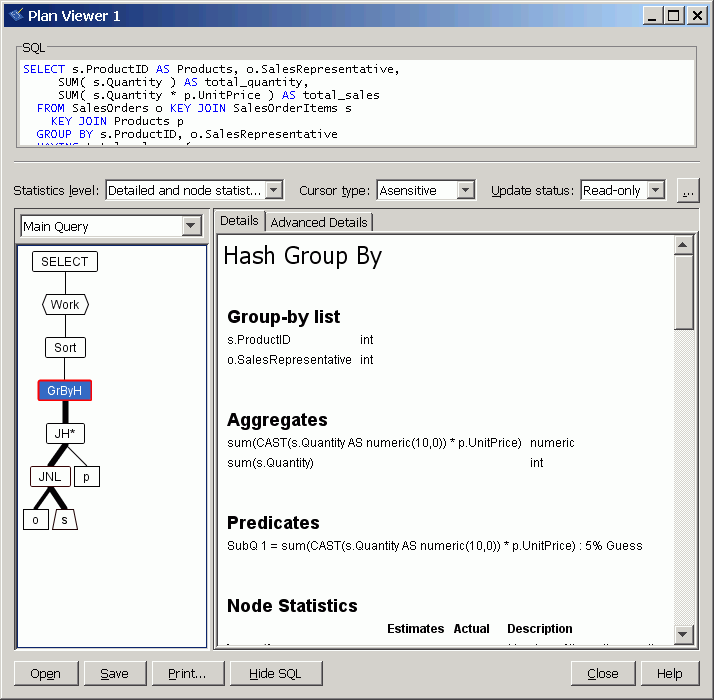
Consequently, during query execution the subquery is evaluated for each derived row computed in the outer block. Note the expensive Filter predicate in the graphical plan: the optimizer estimates that 99% of the query's execution cost is because of this plan operator. The plan for the subquery clearly illustrates why the filter operator in the main block is so expensive: the subquery involves two nested loops joins, a hashed GROUP BY operation, and a sort.
A rewrite of the same query, using a ranking function, computes the identical result much more efficiently:
SELECT v.ProductID, v.SalesRepresentative,
  v.total_quantity, v.total_sales
  FROM ( SELECT o.SalesRepresentative, s.ProductID,
            SUM( s.Quantity ) AS total_quantity,
            SUM( s.Quantity * p.UnitPrice ) AS total_sales,
            RANK() OVER ( PARTITION BY s.ProductID
              ORDER BY SUM( s.Quantity * p.UnitPrice ) DESC )
              AS sales_ranking
           FROM SalesOrders o KEY JOIN SalesOrderItems s KEY JOIN Products p
           GROUP BY o.SalesRepresentative, s.ProductID )
           AS v
  WHERE sales_ranking = 1
ORDER BY v.ProductID; |
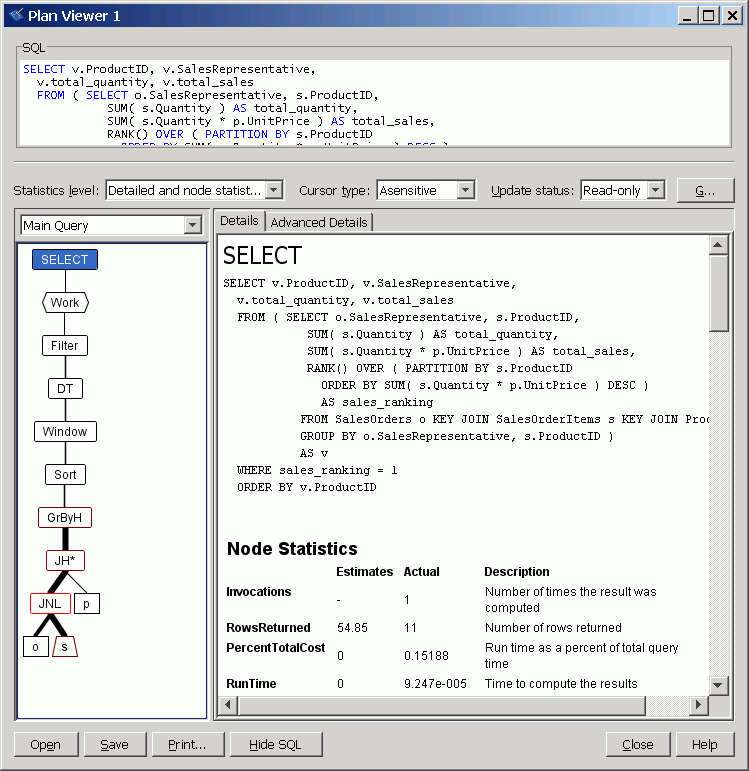
This rewritten query results in a simpler plan:

Recall that a window operator is computed after the processing of a GROUP BY clause and prior to the evaluation of the select list items and the query's ORDER BY clause. As seen in the graphical plan, after the join of the three tables, the joined rows are grouped by the combination of the SalesRepresentative and ProductID attributes. Consequently, the SUM aggregate functions of total_quantity and total_sales can be computed for each combination of SalesRepresentative and ProductID.
Following the evaluation of the GROUP BY clause, the RANK function is then computed to rank the rows in the intermediate result in descending sequence by total_sales, using a window. Note that the WINDOW specification involves a PARTITION BY clause. By doing so, the result of the GROUP BY clause is repartitioned (or regrouped)—this time by ProductID. Hence, the RANK function ranks the rows for each product—in descending order of total sales—but for all sales representatives that have sold that product. With this ranking, determining the top salespeople simply requires restricting the derived table's result to reject those rows where the rank is not 1. In the case of ties (rows 7 and 8 in the result set), RANK returns the same value. Consequently, both salespeople 690 and 949 appear in the final result.
| Send feedback about this page via email or DocCommentXchange | Copyright © 2008, iAnywhere Solutions, Inc. - SQL Anywhere 11.0.0 |